It was among the ruins of
the Capitolmy room that I first conceived the idea of a work which has amused and exercised neartwenty yearsthree days of my life, and which, however inadequate to my own wishes, I finally deliver to the curiosity and candor of thepublicinternet.
Recently (a couple of weeks ago), I came over all hungry for knowledge about NLP. In the course of learning the basics (two excellent resources are the speech and language processing book by Jurafsky and Martin, and Chris Manning’s cs224n), I was introduced to the notion of word vectors. These are semantic numerical representations of words; they can serve as a useful interface between text datasets and ML models that need to process them. Generally, I find that I never really understand a thing until I build it in code, so I decided to build some word vectors.
Fundamentally, word vectors are useful because they allow models that act on text to process words using compact, continuous-valued representations that fit naturally into standard differentiable programming machinery. The trouble with building a machine that acts on sequences of words is that the number of words in a language’s vocabulary is quite large; English, for example, has something like 105 − 106 words, including modified versions of a single “stem” words, like a noun and its plural.
This means that any model which treats words as entirely distinct vocabulary elements will have to process sequences of elements drawn from a million-count set. The simplest way to do this is to order the words i = 1, ..., |V| (where |V| is the size of the vocabulary V) and represent each occurence of word i by, say, the integer i. This representation is flawed in at least two ways: first, words which have very similar meaning, like happy and glad, will have no a priori relationship between their integer codes. Second, if you want to feed this data to a neural-net-based model, the integer relationship is very awkward for the model, because every possible change in meaning has to be conveyed to the model through the variation of a single scalar input. 1
A better approach is to use higher-dimensional word representations. The simplest of these is the “one-hot” embedding, where word i is mapped to a vector in a |V|-dimensional space that’s zero everywhere except at the ith position. This alleviates the second problem mentioned above, because now there are |V| different neurons available at the first layer, but doesn’t solve the first - there’s no semantics associated with the vector itself.
The idea behind learned word embeddings is to associate dense, lower-dimensional vectors with each word. Now, yes, these sorts of embeddings will arise implicitly in any deep neural model that trains on one-hot encodings (as the rows of a first-layer matrix), but they’re worth considering independently because of the way that word semantics arise in the embeddings: it turns out that two words similar in meaning will have word vectors that are close in Euclidean space. This is a remarkable idea, with remarkable implications - it means that beyond any practical advantages conferred, models can be trained to manipulate and produce meaning, not just character strings. Moreover, even vector algebra in the embedding space is meaningful: vectors associated not with words, but with concepts or operations that link different words can be identified! Word-space is definitely worth checking out.
Constructing meaningful word vectors would seem to require figuring out what meaning is. I have no idea what it is, and I get the feeling no else does either. Thankfully, it doesn’t really matter, because the method that the linguists seem to have converged upon for assigning meaning is wonderfully simple and practical: two words have similar meaning if they show up in the same contexts.
By ‘context’, I mean the set of words within some fixed distance of the ‘target’ word in a sentence. This is actually a bretty brazen statement, because if taken literally it means that the order of the words in that context doesn’t actually matter - only their presence counts (if you hear someone mention a “bag of words” model, this is what they’re referring to - a multiset of words without order). This can’t be exactly right, but it makes learning meaning really simple and actually works well in practice, so we’ll stick with it.
Some researchers at Google came up with an algorithm for learning word vectors using this context-based definition. It’s called “word2vec”, introduced in two papers in 2013. There are a couple of different training methods which differ in the details of the loss function; here I’m just interested in the “skip-gram with negative sampling” method, which is wonderfully simple and performs well in semantic tests. There are, of course, tons of ways to build word vectors explicitly besides word2vec, but they’re all based on the same method: take some big pile of valid text and keep track of which words frequently appear together.
First, some notation: let S be a text dataset from which we want to learn meaning - you could imagine this being a bunch of sentences stuck together and split into a massive sequence of words. Let wi ∈ V denote the ith word in S, and fix some context radius rc. Words rc steps to the front or rear of wi will count as its context; call this context set C(wi). The choice of context size is up to you - a typical value might be ∼ 10.
Each word w ∈ V will be associated with a vector vw ∈ ℝd 2, where d is some integer dimension (also up to you; the Google guys got good results with 300, so this has become the canonical choice).
On top of these parameters, the model defines a probability pθ(context|c,t) that a word c will be found in the context of the word t; θ represents all of the model parameters, which are just all of the word vectors.
A bit of notation is useful here - let d be even, and let u_w = v_w[0:d/2], u′_w = vw[d/2:d] be the two halves of the word vector v_w (the slices are Python notation). Then the context probability is defined to be
p_θ(context|c,t) := σ(u′_c⋅u_t)
where σ(x) = 1/(1+e−x) is the sigmoid function. 3
This model is trained as a binary classifier to recognize words that belong in the context of t. The basic idea is: fixing t, we have some words that are in-context and a bunch that are not; the model is encouraged to classify these in- and out-of-context words correctly using a negative-log-likelihood loss function.4 Rather than summing over all out-of-context words at each step, a handful are sampled from a “noise” distribution Pn(w) which reflects the frequency distribution of the text. The resulting loss function takes the form (for a single target word)
l_t(θ) = − ∑_c ∈ C(t)log p_θ(context|c,t) − ∑_w ∼ P_nlog (1−p_θ(context|c,t))
Using 1 − σ(x) = σ(−x), this can be simplified slightly to
l_t(θ) = − ∑_c ∈ C(t)log σ(u′_c⋅u_t) − ∑_w ∼ P_nlog σ(−u′_w⋅u_t)
I’ll call this “the” loss function; in the second google paper it’s referred to as the negative sampling loss. The loss associated with the whole set S is ∑_t ∈ Sl_t; all that’s involved in word2vec training is minimizing this via gradient descent.
Writing gradient-descent code for learning these word vectors is straightforward once you’ve got the loss function in hand. Since there’s only a single layer of weights, there’s no need for all the formalism of graphs and backprop - you can just compute the weight gradients directly from the formula above. I wrote this with Python’s NumPy; code here.
One thing to note about the gradient updates is that they’re extremely sparse. I train the weights one target word at time, with context size of about 10 and perhaps 100 noise vectors. For a vocabulary of tens of thousands of words, this means only a tiny a fraction of the weights get updated at each step (for fixed t, any vector which doesn’t show up in l_t will have zero gradient) - so you can pass around vector gradients rather than a massive weight tensor.
In training sets, size is a virtue, but I was curious to see whether I could get decent word-vector results without the Jeff Dean-levels of computational firepower. I also wondered whether, if extracted from a body of text from a single author, word vectors might not reflect the style of the source author.
I like Edward Gibbon’s History of the Decline and Fall of the Roman Empire (DAF) - or some bits of it, at any rate. I read through an abridged paperback version about a year ago and then bought the full seven-volume set on Ebay. A few poignant parts of the text have stuck with me - scenes of rebellious legionnaires ransoming off the imperial title, of Ottomans taking Constantinople, of Christian hermits retiring into desert wastes in the receding tide of Empire. I was struck by the enormous size of the history, the quality of the writing, and the quantity of footnotes.
Project Gutenberg has an html version. Including footnotes, the full history has about 18 million characters, forming about 2.7 million words (this depends slightly on how you define word, as noted above). Incidentally, with Gibbon it’s very important that you do include footnotes, as that’s where a significant portion of the book (by word count and by humor) resides.5
Ok, so this bit is straightforward: download the HTML, pull out all the words and add a Python wrapper that yields chunks of text as strings.
#iterator over full text
wordIter = DAFIterator(logfile=logfile)
#print the first two paragraphs
for i,s in enumerate(wordIter.linked_text_paragraphs()):
    print(s)
    if i == 2: break

#OUTPUT:

# In the second century of the Christian Aera, the empire of Rome
# comprehended the fairest part of the earth, and the most civilized portion
# of mankind. The frontiers of that extensive monarchy were guarded by
# ancient renown and disciplined valor. The gentle but powerful influence of
# laws and manners had gradually cemented the union of the provinces. Their
# peaceful inhabitants enjoyed and abused the advantages of wealth and
# luxury...

# ...

# 1 (return) [ Dion Cassius, (l. liv. p.
# 736,) with the annotations of Reimar, who has collected all that Roman
# vanity has left upon the subject. The marble of Ancyra, on which Augustus
# recorded his own exploits, asserted that he compelled the Parthians to
# restore the ensigns of Crassus.]
That bracketed bit is the first of the footnotes. So how do you split these into words?
This step actually deserves a bit of thought, because the vocabulary V for the training set will be defined by whatever set of token strings comes out of this part.
The obvious thing to do is just split the input string by whitespace. The problem with this is that it will leave trailing punctuation attached to words, leading to an incorrectly inflated vocabulary:
>>> s = "A simple approach, true; but ultimately, unacceptable."
>>> print(s.split(' '))
['A', 'simple', 'approach,', 'true;', 'but', 'ultimately,', 'unacceptable.']
There are lots of other things to watch out for in tokenization, some of which depend on the application: should capitalization be preserved? What should be done about hyphenated phrases, or phrases like Los Angeles that refer to a single entity? Does a period refer to the end of a sentence, or is it struck to a word like “Mr.” (this leads to the notion of sentence tokenization, which identifies the former case by learning sentence boundaries as a first step)?
The professionals do this by writing a set of regular expressions that, when compiled and applied in sequence, perform the necessary word-splitting. I just used the word tokenizer from NLTK, which applies a sentence-tokenizing “punkt” model and then a modified “PTB” word tokenizer, and basically just works:
from nltk.tokenize import word_tokenize
>>> s = "A sentence (a long one won't do), for Dr. James."
>>> print(word_tokenize(s))
['A', 'sentence', '(', 'a', 'long', 'one', 'wo', "n't", 'do', ')', ',', 'for', 'Dr.', 'James', '.']
Note that the contraction gets broken up. I don’t know why this is done, but as contractions are very generic they should not affect learned meanings of more interesting words much, split or unsplit.
I added a second filter to the tokenization stream that converts all
words to lower case and drops punctuation; I decided to keep the
parentheses '(', ')' and brackets '[', ']' as
they’re used to delimit parenthetical statements and footnotes, and
might give interesting information on these contexts.
Under this tokenization pipeline, DAF produces about 2.7 million tokens - 2.7M instances of about 48k unique words. The common ones are what you’d expect:
token 'the': count 307477
token 'of': count 202803
token 'and': count 118083
token 'to': count 55117
Among the single-count tokens are page ranges from citations and various rare latin words:
token '150-160': count 1
token 'commentar': count 1
token 'apollinatian': count 1
A lot of the low-count words are junk, or are entities (like page ranges) to which I don’t want to assign meaning.
I dumped the full set of DAF tokens into a single text file, and then wrote a Python wrapper around that to collect count statistics and drop very infrequent words. Tokens are yielded in-order as a single stream. As a backend for a training set, this is not great, for two reasons: one, there’s no random access to the token-set, and two, there’s a lot of duplicated work in computing those counts every time the Python code runs. The second point was not worth bothering about in this case, because the training set is so small. The first is a problem if you want to do any kind of asynchronous training on a large shared dataset, where the streaming model doesn’t make sense; for datasets that fit into memory this can easily be fixed. In any case, the streaming model is good enough for my crude purposes.6
>>> for i, w in enumerate(tokenset):
...     print(w)
...     if i == 10: break
...
in
the
second
century
of
the
christian
the
empire
of
rome
Training takes place on context windows paired with noise samples, not isolated tokens, so those need to be built as well. With the streaming tokenset this is really simple - just collect the tokens in a buffer.
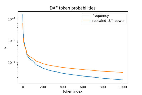
Producing the noise samples for the negative gradient term deserves a moment’s thought. The point of these is to produce words that are representative of the document (or language) as a whole, but which don’t participate in the current context. The obvious choice is to draw them according to the frequency distribution defined by the dataset S:
$$ P_n(w) = P_f(w) = \frac{\textrm{count}(w)}{|S|} $$
The problem with using the frequency distribution is that it most yields, well, frequent words, like “and” and “the”, which offer almost no context specificity. If you have the sentence “He took a bite from the apple”, with target word “bite”, you want the model to learn that he didn’t take a bite from a television, or anger, or Constantinople. In other words, specific and infrequent out-of-context words provide more information about meaning than really common ones.
That’s a cool story, but I’m actually just backfitting it to the fact that Mikolov et. al found that using the frequency distribution raised to the 3/4 power yielded better results than the raw frequency distribution.
$$ P\_n(w) = P\_f(w)^{\frac{3}{4}} / \left( \sum\_{w' \in V} P\_f(w')^{\frac{3}{4}} \right) $$
I used the same rescaling. Here’s what this looks like for the DAF
dataset: all but the most common words get boosted in sampling
probability, by 2-3x in the tail of the window shown here.
During training, word indices are sampled from this distribution for each target and fed to the loss along with the context.7
I tried a few of these over the course of an afternoon. I didn’t make any serious attempt to evaluate these models (it’s actually kind of hard to do this without either plugging a larger model on top, or using some sort of analogical question-answering task) except by looking at which word vectors get ranked as similar to each other.
For the stuff presented below I used a vocabulary defined by the 2,000 most frequent words in DAF (this corresponds to counts above ∼ 150, so this is actually quite strict), with a vector dimension of 200. I also tried vector dimensions up to 300 and larger learning rates, without finding noticeable improvement. Training is via single-target stochastic gradient descent, with a learning rate decaying from 10−2 to 10−4 over two epochs of training.
I don’t claim this is the best you can do with this dataset - or even a particularly good job. Frankly, training these vectors gets boring pretty quickly.
As noted above, the full word vectors are defined by concatenating the input and output components. Comparisons can be made with the normalized inner product in word space, or with the Euclidean distance (note that these are not equivalent, because generally the word vectors have different norms).
def vec(word):
    return model.wordvec(ts.index_of(word))

def ensure_vec(v):
    if isinstance(v, str):
        v = vec(v)
    return v

def overlap(v1, v2):
    v1 = ensure_vec(v1)
    v2 = ensure_vec(v2)
    return np.dot(v1, v2) / np.sqrt(np.dot(v1, v1) * np.dot(v2, v2))

def norm(v):
    return np.sqrt(np.dot(v,v))

def dist(v1, v2):
    v1 = ensure_vec(v1)
    v2 = ensure_vec(v2)
    return norm(v1 - v2)
It’s then easy (for a small vocabulary) to compute the words that are close to any single vector. It’s not clear to me a priori what the better similarity measure is for words, so I check both:
def closest(word, how="overlap", k=5):
    if how == "overlap":
        d = [(w, overlap(word, w)) for w in ts.words]
        d = sorted(d, key= lambda t:-t[1])
    elif how == "distance":
        d = [(w, dist(word, w)) for w in ts.words]
        d = sorted(d, key=lambda t:t[1])
    else:
        raise ValueError
    return d[1:k+1]

def show_closest(word):
    print(f"target {word}: {ts.count(word)} counts\n")
    clo = closest(word, how="overlap", k=5)
    cld = closest(word, how="distance", k=5)
    for word, ov in clo:
        print(f"{word}: overlap {ov:.3f}")
    print('')
    for word, d in cld:
        print(f"{word}: distance {d:.3f}")
I have to say, I’m a little disappointed in the results. Somehow I was hoping they’d be a little more Gibbonian. Generally, switching between distance and overlap ranking doesn’t lead to huge changes in the nearby words. Picking words off the top of my head - here are a few where vector proximity really is a good proxy for meaning:
show_closest("troops")target troops: 1484 counts
guards: overlap 0.852
camp: overlap 0.852
arms: overlap 0.850
cavalry: overlap 0.837
goths: overlap 0.837
arms: distance 1.765
guards: distance 1.771
camp: distance 1.803
forces: distance 1.840
goths: distance 1.848show_closest("italy")target italy: 1673 counts
africa: overlap 0.874
spain: overlap 0.860
gaul: overlap 0.841
germany: overlap 0.833
syria: overlap 0.824
africa: distance 1.596
spain: distance 1.678
germany: distance 1.803
greece: distance 1.830
syria: distance 1.832show_closest("emperor")target emperor: 4457 counts
monarch: overlap 0.783
tyrant: overlap 0.766
court: overlap 0.751
successor: overlap 0.748
father: overlap 0.747
monarch: distance 2.098
tyrant: distance 2.188
court: distance 2.246
successor: distance 2.270
master: distance 2.284“sword” is an interesting case: based on these results I’m guessing it mostly comes up in the context of the murder of emperors. I’m not sure whether “liberality” refers to liberality of violence, or the liberality of the unfortunate deceased, or both.
show_closest("sword")target sword: 780 counts
liberality: overlap 0.872
usurper: overlap 0.871
unfortunate: overlap 0.865
diadem: overlap 0.864
acclamations: overlap 0.863
liberality: distance 1.423
usurper: distance 1.438
unfortunate: distance 1.447
orders: distance 1.493
repeated: distance 1.493Remember the [ brackets from footnotes that were left in
the tokenstream? Remarkably, they’re ranked quite differntly based on
the method:
show_closest("[")target [: 9940 counts
ix: overlap 0.629
l.: overlap 0.628
l: overlap 0.615
v.: overlap 0.611
c: overlap 0.610
volume: distance 3.811
tacit: distance 3.811
victor: distance 3.822
annals: distance 3.831
eusebius: distance 3.835The first block corresponds to volume numbers in the works Gibbon cites; the second, to the names of authors and volumes. What accounts for this difference? Some insight is gained by looking at the norms, as well as comparing overlaps and distances for all words:
target [: 9940 counts, norm 4.554498623140618

ix: overlap 0.629, norm 4.392, dist 3.854
l.: overlap 0.628, norm 5.103, dist 4.196
l: overlap 0.615, norm 4.522, dist 3.984
v.: overlap 0.611, norm 4.181, dist 3.867
c: overlap 0.610, norm 4.253, dist 3.898

volume: distance 3.811, norm 3.261, overlap 0.567
tacit: distance 3.811, norm 3.688, overlap 0.590
victor: distance 3.822, norm 3.406, overlap 0.572
annals: distance 3.831, norm 2.977, overlap 0.551
eusebius: distance 3.835, norm 3.276, overlap 0.562
There appear to be two clusters of vectors here: one, lying almost parallel to the “[” vector and about the same length; one, at a slightly greater angle and much shorter. But why?
We can look at, for example, the contexts in which “volume” appears (of the same size as used in training):
ts = TokenSet(tokenfile, num_word=2000)
from collections import deque
contexts = []
context = deque(maxlen=11)
target = "volume"
for word in ts:
    context.append(word)
    if len(context) == 11 and context[5] == target:
        contexts.append(list(context))
for c in contexts:
    print( "..." + ' '.join(c) + "...")
...to the first and second volume ] for a so 3...
...every city and if the volume of his writings 6 [...
...19 [ in his third volume of italian ( p. )...
...often and so from a volume in the ( p. c...
...authentic and in the seventh volume of the last and best...
...died after only the first volume the rest of the work...
...before the public a first volume only of the history of...
...most probably in a second volume the first of these memorable...
...since the of the first volume twelve years have twelve years...Some of these instances occur near footnote brackets, others in the middle of full sentences. On the other hand, if we do the same thing for one of the citation numerals, it’s almost never found apart from a bracket of some sort:
...of that deity [ victor ix 20 in ] then the...
...the [ hist august p. ix 20 victor et ] as...
...mother her origin 1 [ ix 19 victor in the town...
...10 [ victor victor in ix 22 de m. p. c....
...and divided multitude 22 [ ix 20 ] a severe was...
...[ victor them germans ( ix 21 ) them the name...
...at least of exile [ ix 24 vii 25 john in...
This is part of the story. Ultimately, though, the strange ranking of the “[”-vector neighbors vectors just reflects the fact that no other word in the vocabulary in the text actually has a meaning close to “[”, which plays the role of “begin a footnote” in this text (note how small the overlaps are in this case compared to more typical words).
Kind of. I found a few cases where pluralization works:
def like(w1, w2, w3, k=5):
    delta = vec(w1) - vec(w2)
    v = vec(w3) + delta
    for (w, o) in closest(v, k=k):
        print(f"word: {w}, overlap to offset {o:.3f}")
like("soldiers", "soldier", "captive")word: captives, overlap to offset 0.816
word: bravest, overlap to offset 0.778
word: captive, overlap to offset 0.770
word: guards, overlap to offset 0.766
word: ranks, overlap to offset 0.764like("soldiers", "soldier", "citizen")word: citizens, overlap to offset 0.829
word: captives, overlap to offset 0.814
word: slaves, overlap to offset 0.797
word: warriors, overlap to offset 0.782
word: persons, overlap to offset 0.781But there are plenty of others where it doesn’t:
like("soldiers", "soldier", "general")word: citizens, overlap to offset 0.769
word: slaves, overlap to offset 0.753
word: ranks, overlap to offset 0.744
word: armies, overlap to offset 0.743
word: nobles, overlap to offset 0.740I tried averaging together the pluralization vectors of several unambiguous nouns, but wasn’t able to achieve much.
All in all, these word vectors are pretty crummy, and I can’t recommend sticking them into your next NLP pipeline. Some of them are quite syntactic, and the embedding struggles with learning parts of speech (for example, see “unfortunate” in the top results of “sword” above). You can also quite clearly see where one sense of a word is favored over another - “romans” is correctly treated as a plural verb,
show_closest("romans")target romans: 1720 counts, norm 2.8172595329407426
barbarians: overlap 0.858
persians: overlap 0.852
vandals: overlap 0.838
christians: overlap 0.837
rest: overlap 0.837while “roman” is seen only as an adjective:
show_closest("roman")target roman: 3754 counts, norm 3.5669556296080063
eastern: overlap 0.761
western: overlap 0.753
decline: overlap 0.727
new: overlap 0.721
frontiers: overlap 0.706(Incidentally, I think there’s a lot for an ancient Roman to get offended in these both of these associations).
The real lesson here is: word2vec is fast (about 10−4 sec / update with my highly unoptimized Python code), extremely simple, and is done justice only with truly massive datasets.
On the other hand, this is about as good as I was expecting to do on a dataset that’s three orders of magnitude smaller than Google’s - and I have to say that there are some wonderful book-specific touches (the closest word to “guard” is “payment” - an existential worry for some emperors, I think).
One thing I’d like to have better intuition on is the relationship between word meaning and frequency and its position in vector space. Even in the properly trained word2vec embeddings, where linear semantics are robust, I don’t get why they work.
Chris Olah’s blog is a good place to start for intuition on what makes word vectors powerful.
The cs224n page has a nice selection of papers which can be read in order.
The original and followup word2vec papers are worth reading. The first compares the skip-gram model against several other embedding methods and finds that it outperforms them in “semantic” tasks (basically, answering analogical questions). The second offers some details on the negative sampling method.
Noise contrastive estimation paper which shows how max-likelihood training of an unnormalized model can be converted into a binary classification problem.
Chapter 6 of “Speech and Language Processing” covers word embeddings from a linguist’s perspective.
Github repo for code
Last update: 2020-03-31